Warning: package 'downloadthis' was built under R version 4.3.3Case Study: Healthy-Sick-Dead Disease Model
Introduction
This case study will build a decision model to analyze strategies to prevent and treat a noncommunicable disease.
For this hypothetical disease, these high-risk individuals start off healthy and can develop a chronic disease. They stay sick until death. Individuals also experience mortality from other causes.
A state transition “bubble” diagram of the model you will build is shown below:

Policy Decision Problem
Suppose there is a new treatment that can be taken to reduce the likelihood of disease progression. This treatment reduces the probability of death from disease, and slightly increases quality of life (lowers the disability weight) in the sick state. However, this is an expensive treatment.
The Ministry of Health has empowered your team to conduct an economic evaluation to investigate the costs and benefits of the status quo (i.e., do nothing) vs. adopting the use of treatment.
Model Parameters
Relevant model parameters are summarized in the tables below:
State Transition Probabilities
| Name | Value | Description |
|---|---|---|
| p_start_healthy | 1 | Probability of starting in the healthy state |
| p_sick | 0.6 | Probability of disease onset |
| p_death_oc | Age-dependent life table data. | Probability of death from other causes. |
| p_death_disease | 0.05 | Probability of death from progressive disease. |
Costs
| Name | Value | Description |
|---|---|---|
| c_healthy | 0 | Annual (cycle) cost of healthy state. |
| c_sick | 3,500 | Annual (cycle) cost of disease state. |
| c_treatment | 40,000 | One-time cost of disease treatment (occurs at point of transition from Healthy to Sick). |
Disability Weights
| Name | Value | Description |
|---|---|---|
| dw_sick | 0.15 | Quality-of-life (QoL) weight for disease health state. |
| dw_sick_treated | 0.13 | Quality-of-life (QoL) weight for disease health state if treated. |
Other Parameters
| Name | Value | Description |
|---|---|---|
| initial_age | 0 | Initial age of modeled cohort |
| rr_treatment | 0.60 | Treatment Strategy: Relative risk reduction in probability of death from progressive disease. |
| r_disc_health | 0.03 | Annual discount rate: health outcomes. |
| r_disc_cost | 0.03 | Annual discount rate: cost outcomes. |
| t | 110 | Horizon of the model |
| yll_t | Age-Varying | Years of Life Lost discounted from time of death |
Status Quo Scenario
Your first objective is to build a status quo or “do nothing” strategy based on the description and parameters defined above. This is a strategy in which there is no additional treatment.
To get you going, we have built out the beginnings of a model based on an alive-dead model with age-specific background mortality rates. You can download this model at ADD LINK. The image below shows the structure of this model:

Add Health States and Transitions
When you reach the end of the branch, select the chance node you would like to turn into a state transition, right click, select Change to State Transition. This will give you the blue arrow
 . On the right of this arrow, you can find a dropdown menu with the different health states you specified. Select the health state this part of the cohort will transition to.
With this button
 you can align the end nodes.
It is common practice in teaching decision modeling to model events sequentially. Suppose, for example, that an individual can experience the following events from a diseased state:
-   Die from disease (Event A)
-   Die from background causes (Event B)
-   Survive
The image below shows two alternative approaches to modeling these events. Panel A uses a non-sequential approach in which events in a cycle are not conditional on other events not occurring. Panel B, by comparison, first considers death from Event A. Conditional on surviving A, it then considers death from Event B.

If you are converting rates to probabilities using standard formulas (e.g., \(1-\exp(-r)\)) you should use a sequential approach where only two events are considered at at time (Panel B). This ensures that the converted probabilities work correctly.
If you are using transition probabilities derived from embedding the transition probabilities from the underlying transition rate matrix, as we covered in lecture, you do not need to undertake the sequential approach: you can use the approach in Panel A, though you will also need to make sure that your model structure captures all non-zero probabilities in your transition probability matrix.
For the remainder of this case study we will model the disease progression using the sequential approach (e.g., the approach in Panel B).
Your Markov model should now look like this:

Define Transition Probabilities
After inputting the transition probabilities, your Markov model should look like this:

Define Outcomes
Go to Model > Properties > select the Analysis tab.
Check that you have the outcomes for costs and Years Lived with Disability (YLD)
The “Analysis Type” should be set to Expected Value (EV)
We want to reset the objective to minimize. In DALYs, we want to decrease the YLDs and YLLs.

Next, in the model itself, define the following cycle-specific payoffs based on the values in the tables above. Many of these parameters are already defined for you in the parameters tab in the Amua model:
Costs and YLDs in Healthy state
Costs and YLDs in the Sick state
There are no costs are YLDs for the Dead state
After inputting the outcomes, your Markov model should look like this:

Define Cycle Adjustments and Discounting
- Go to Model > Properties > select the Markov tab.
- Select the “Half-Cycle Correction” option.
- Select the “Discount Rewards” option and enter the discount rates shown in the tables above.
- Click “OK”
Treatment and Prevention Strategies
Our next objective is to build out the treatment strategy. Fortunately, we have already done most of the work to add them – we just need to copy and paste the Status Quo strategy, then adapt with additional parameters as needed.
Treatment Strategy
- Right click on the
 Markov symbol next to the Status Quo strategy name, then select “Copy”
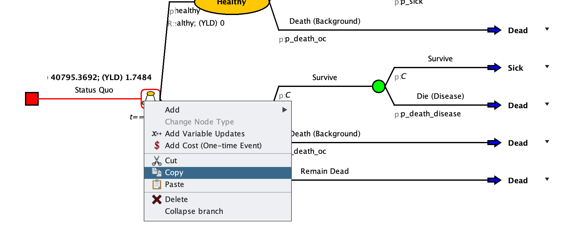
Right click on the red square and select “Paste.” This will create a copy of the Status Quo strategy. Hit the OCD button to organize things again
Rename the new strategy to “Treatment” and adapt the transition probabilities using the prevention strategy parameters defined in the tables above (and in the Amua model parameters).
- Make sure to multiply
p_death_diseaseby the relative risk reduction each time it appears in the branches!
- Make sure to multiply
Update the utility payoff for the progressive disease state using
dw_sick_treatedInclude the one-time treatment cost at the time of transition from mild to progressive disease (see below)
To define a one time treatment: We will add this cost by assigning a one-time cost at the time an individual transitions to the Death (Disease) state from the Progressive disease state. You can add this one-time cost by right-clicking on the transition node
after “Dead (Disease)” in the Progressive Disease health state, and then clicking on  Add Cost.
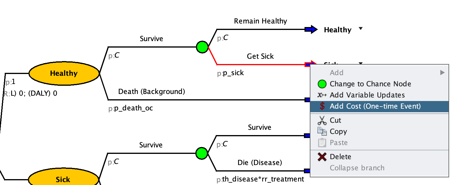
After inputting the outcomes, your treatment branch should look like this:
.png)